Quick Start Guide
This guide will get you running SOLWEIG-GPU in minutes.
Basic Workflow
Prepare input rasters
Prepare meteorological data
Run simulation
Analyze outputs
Sample Data
Sample data is available in Zenodo.
Example 1: Using Your Own Met Data
The simplest way to run SOLWEIG-GPU:
from solweig_gpu import thermal_comfort

thermal_comfort(
    base_path='/path/to/your/data',
    selected_date_str='2020-08-13',
    building_dsm_filename='Building_DSM.tif',
    dem_filename='DEM.tif',
    trees_filename='Trees.tif',
    use_own_met=True,
    own_met_file='met_data.txt'
)
Required Input Files
Place these in your base_path directory (or pass complete paths to rasters in other locations):
Building_DSM.tif - Building + terrain heights
DEM.tif - Digital elevation model (terrain only)
Trees.tif - Vegetation heights
met_data.txt - Meteorological forcing data
To write outputs to a different folder, set base_path to that directory and give full paths for Building DSM, DEM, Trees, and land cover (optional).
Met Data Format
Create a text file with hourly data using the UMEP MetProcessor.
Example 2: Using ERA5 Data
Download ERA5 from the Climate Data Store and run:
from solweig_gpu import thermal_comfort

thermal_comfort(
    base_path='/path/to/data',
    selected_date_str='2020-08-13',
    use_own_met=False,
    data_source_type='ERA5',
    data_folder='/path/to/era5/files',
    start_time='2020-08-13 00:00:00',
    end_time='2020-08-14 23:00:00'
)
When using ERA-5 dataset, the package can find the corresponding data for start_time and end_time. For example, if ERA-5 data is downloaded from 2020-08-13 00 UTC to 2020-08-14 23 UTC and the model is to be run from 2020-08-13 06 UTC to 2020-08-14 05 UTC, the package can select data from 2020-08-13 06 UTC to 2020-08-14 05 UTC by itself (selected_date_str = ‘2020-08-13’, start_time = ‘2020-08-13 00:00:00’, and end_time = ‘2020-08-14 23:00:00’)
start_time and end_time must be in UTC. The package will automatically convert to local time based on the geographic location of your study area.
Example 3: Using WRF Output
from solweig_gpu import thermal_comfort

thermal_comfort(
    base_path='/path/to/data',
    selected_date_str='2020-08-13',
    use_own_met=False,
    data_source_type='wrfout',
    data_folder='/path/to/wrfout/files',
    start_time='2020-08-13 06:00:00',
    end_time='2020-08-14 05:00:00'
)
When using wrfout, the start_time and end_time should be the first and last time stamps in the wrfout dataset. The package won’t compare the selected start_time and end_time to the wrfout file timestamps and automatically fetch the corresponding data.
start_time and end_time must be in UTC. The package will automatically convert to local time based on the geographic location of your study area.
Note for Windows Users
On Windows, Python uses the spawn start method for new processes: each worker re-imports your script. Without guarding the entry point, a top-level call to thermal_comfort() would run again in every child process, causing repeated execution and failures (e.g. BrokenProcessPool). Always call thermal_comfort() inside a main() function and use if __name__ == "__main__": (see example below).
from solweig_gpu import thermal_comfort
import multiprocessing as mp

def main():
    thermal_comfort(
        base_path='/path/to/input',
        selected_date_str="2020-08-13",
        building_dsm_filename="Building_DSM.tif",
        dem_filename="DEM.tif",
        trees_filename="Trees.tif",
        landcover_filename="Landcover.tif",
        tile_size=1000,
        overlap=100,
        use_own_met=False,
        own_met_file='/path/to/met.txt',  # placeholder; ignored when use_own_met=False
        start_time="2020-08-13 06:00:00",
        end_time="2020-08-14 05:00:00",
        data_source_type="era5",
        data_folder='/path/to/era5_or_wrfout',
        save_tmrt=False,
        save_svf=False,
        save_kup=False,
        save_kdown=False,
        save_lup=False,
        save_ldown=False,
        save_shadow=False,
    )

if __name__ == "__main__":
    mp.freeze_support()
    main()
Command-Line Usage
# Using own met data
thermal_comfort \
    --base_path /path/to/data \
    --date 2020-08-13 \
    --tile_size 1000 \
    --use_own_met True \
    --own_metfile /path/to/ownmet.txt

# Using ERA5
thermal_comfort \
    --base_path /path/to/data \
    --date 2020-08-13 \
    --tile_size 1000 \
    --overlap 100 \
    --use_own_met False \
    --data_source_type ERA5 \
    --data_folder /path/to/era5 \
    --start "2020-08-13 00:00:00" \
    --end "2020-08-14 23:00:00"
Configuration Options
Tile Size
Adjust based on GPU memory:
thermal_comfort(
    base_path='/path/to/data',
    selected_date_str='2020-08-13',
    tile_size=1000,  # Smaller = less memory, more tiles
    overlap=100,     # Overlap for shadow continuity
    ...
)
Guidelines:
8GB GPU:
tile_size=1000-200016GB GPU:
tile_size=2000-400032GB GPU:
tile_size=4000+
Output Options
thermal_comfort(
    base_path='/path/to/data',
    selected_date_str='2020-08-13',
    save_tmrt=True,      # Mean radiant temperature
    save_svf=True,       # Sky view factor
    save_kup=True,       # Upward shortwave
    save_kdown=True,     # Downward shortwave
    save_lup=True,       # Upward longwave
    save_ldown=True,     # Downward longwave
    save_shadow=True,    # Shadow maps
    ...
)
GUI Usage
To launch the GUI:
conda activate solweig
solweig_gpu_gui
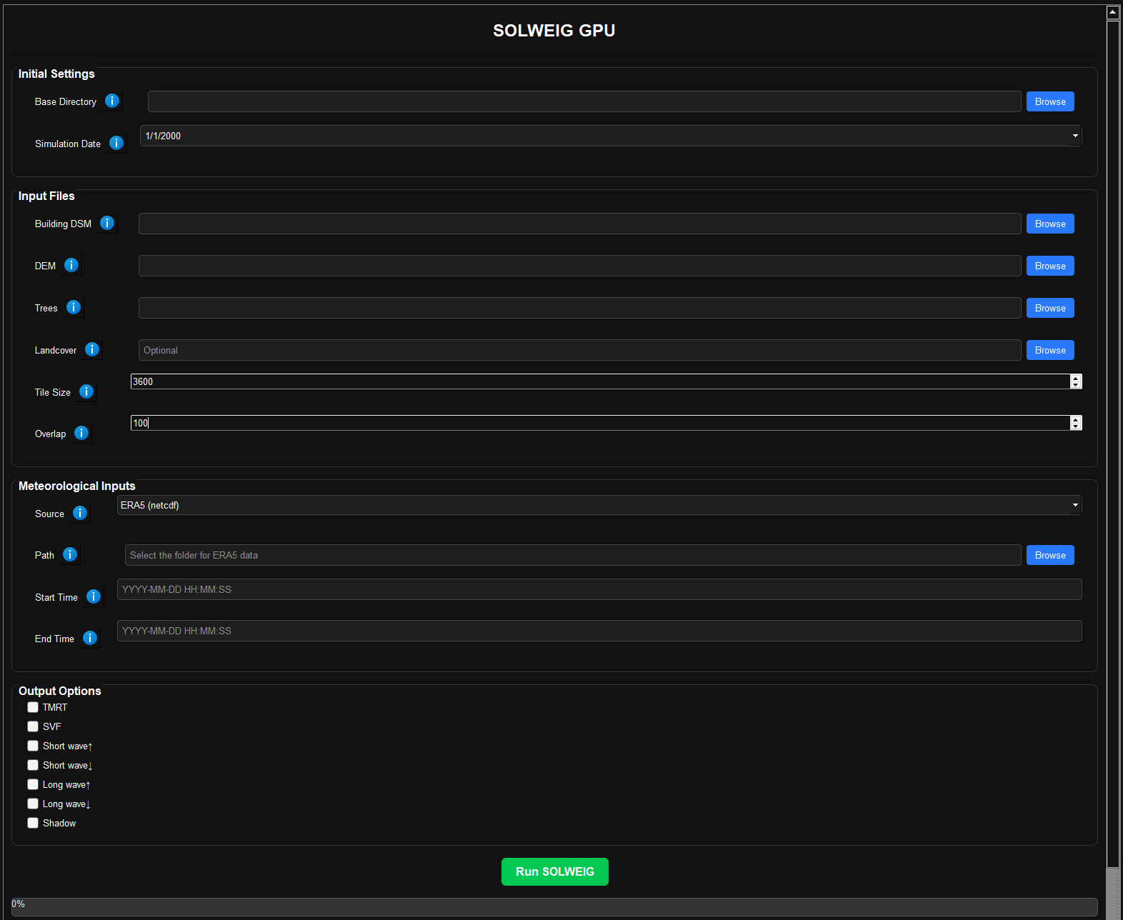
GUI Workflow
Select the base path containing input datasets.
Choose the Building DSM, DEM, Tree DSM, and Land cover (optional) raster files.
Set the tile size (e.g., 600 or 1200 pixels).
Select a meteorological source (
metfile,ERA5, orwrfout):If
metfile: Provide a.txtfile.If
ERA5: Provide a folder with both instantaneous and accumulated files.If
wrfout: Provide a folder with WRF output NetCDF files.
Set the start and end times in UTC (
YYYY-MM-DD HH:MM:SS).Choose which outputs to generate (e.g., Tmrt, UTCI, radiation fluxes).
Output will be saved in
output_folder/, with subfolders for each tile (keyed by tile origin, e.g.0_0,1000_0).
Output Files
Results are saved in {base_path}/output_folder/{tile_key}/:
output_folder/
├── 0_0/
│   ├── UTCI_0_0.tif       # Thermal comfort index (multi-band, one per hour)
│   ├── TMRT_0_0.tif       # Mean radiant temperature (if save_tmrt=True)
│   ├── SVF_0_0.tif        # Sky view factor (if save_svf=True)
│   └── ...
├── 1000_0/
│   └── ...
See Outputs for full details. Each time-varying .tif is a multi-band raster (one band per hour).
Calling pipeline stages separately
You can run the workflow in three steps: preprocess → run_walls_aspect → run_utci_tiles. This is useful to run only a subset of tiles or to reuse preprocessed data. The CLI and GUI still use the one-shot thermal_comfort(); no changes there.
from solweig_gpu import preprocess, run_walls_aspect, run_utci_tiles

preprocess_dir = preprocess(base_path=base_path, selected_date_str=date_str, ...)
run_walls_aspect(preprocess_dir)
run_utci_tiles(base_path=base_path, preprocess_dir=preprocess_dir, selected_date_str=date_str, ...)
For full parameter lists and examples (including running only specific tiles), see Developer Guide – Pipeline stages and API Reference.
Next Steps
Developer Guide (pipeline stages, architecture)